A. Background
The Open Powerlifting initiative attempts to create an accurate and open archive of all powerlifting meet data throughout the world. As someone who recently started competing again after a six year delay from powerlifting, I often mess around with the Open Powerlifting data as it’s of personal interest. Most of the anlysis that I’ve done to date has been posted on other platforms, but I decided to start expanding on that analysis on this blog. For this first post, I’m going to investigate how personal factors such as gender, weight, and age impact total weight lifted.
B. First Steps
The data from the Open Powerlifting project can be acquired from the following location.
https://www.openpowerlifting.org/data
Let’s start by importing the data and required packages for this analysis.
library(data.table)
library(ggplot2)
library(lubridate)
library(stringr)
library(zoo)
library(rms)

dat <- fread("openpowerlifting.csv")

dat[1:3]
Each row in this data set represents the lifts for a lifter at a specific meet. If a lifter has competed in five different meets, they will have five different rows that describe everything from their age, body weight, federation, and so forth.

C. Data Cleaning and Feature Engineering
There is a date column in the dataset. However, I’ve created some new date columns so that I can visualize patterns over time.
dat[, Date_Year := lubridate::year(lubridate::ymd(Date))]
dat[, Date_Month := lubridate::month(lubridate::ymd(Date))]
dat[, Date_YearMonth := ymd(paste(Date_Year, "-", Date_Month, "-", "01", sep=""))]
For this analysis, we will only look a full powerlifting meets in the United States from 01/2000 through the end of 06/2019.
## only look at full powerlifting meets in the united states

mydat = dat[, Date := lubridate::ymd(Date)][
             MeetCountry %in% c("USA") &
             Event %in% c("SBD") &
             lubridate::year(lubridate::ymd(Date)) >= 2000 &
             Date_YearMonth <= lubridate::ymd("2019-05-01"),]
An unique identifier was created for each lifter based on their name and gender. While this works for most entries in the data set, please note that some lifters with common names will end up being grouped together.
## lifter unique id

mydat[, lifter_id := .GRP, by=.(Name, Sex)]

lifter_cnt = mydat[, .(num_meets = .N), by=lifter_id]

mydat = mydat[lifter_cnt,  nomatch=0, on = 'lifter_id']

mydat[, lifter_experienced := ifelse(num_meets >= 10, 1, 0)]
An unique identifier was created for each powerlifting meet based on the meet name, federation, date, and meet country. This new column will be used to distinguish between small and big meets, with those meets containing more than 150 lifters being classified as big.
## small or big meet

mydat[, meet_id := .GRP, by=.(Federation, Date_Year, MeetCountry, MeetState, MeetName)]

meet_cnt = mydat[, .(num_lifters = .N), by = meet_id]

mydat = mydat[meet_cnt, nomatch=0, on = 'meet_id']

mydat[, big_meet := ifelse(num_lifters >= 150, 1, 0), ]
Another thing I wanted to explore was the proportion of women across all meets. To do that, I used the unique meet identifier to find the proportion of women who competed in that meet.
## proportion of women per meet

women_cnt = mydat[, .(N = .N), by = .(meet_id, Sex)]
mydat = mydat[women_cnt, nomatch=0, on = 'meet_id']

mydat[, prop_women := round(N/sum(N),2), by = .(meet_id)]

mydat = [Sex == "F",]

mydat[, Sex := NULL][, N := NULL][,

mydat[, prop_women_high := ifelse(prop_women >= 0.40, 1, 0)]
Another thing I wanted to explore was the proportion of older lifters (50+) across all meets. To do that, I used the unique meet identifier to find the proportion of lifters who were 50 year old and older that competed in the meet.
agebreaks <- c(0, 20, 35, 50, 500)
agelabels <- c("0-20", "21-35", "36-50","51+")

mydat[!is.na(Age), AgeBucket := cut(Age,
                                    breaks = agebreaks,
                                    right = FALSE,
                                    labels = agelabels)]
## proportion of older lifters in a meet

old_cnt = mydat[!is.na(Age), .(N = .N), by = .(meet_id, AgeBucket)]

mydat = mydat[old_cnt, nomatch=0, on = 'meet_id']

mydat[, prop_old := round(N/sum(N),2), by = .(meet_id)]

mydat = mydat[AgeBucket == "51+",]

mydat[, AgeBucket := NULL][, N := NULL]

mydat[, prop_old_high := ifelse(prop_old >= 0.10, 1, 0)]
We will only examine the entries from lifters who have competed in 50 or less meets.
mydat = mydat[num_meets <= 50,]
D. Exploratorty Data Analysis
Let’s start by looking at the total number of full powerlifting meets occuring by month. Meets from two federations were filtered out because they are Texas high school powerlifting federations and account for a lot of meets where the lifters were underage. We can see that there has been a substantial increase in the number of powerlifting meets occuring since 2010.
mydat[!Federation %in% c("THSPA","THSWPA"), .N, by = .
      (Date_YearMonth, MeetName)][,
      .N,  by = .(Date_YearMonth)][order(Date_YearMonth)][] %>%
ggplot(., aes(Date_YearMonth, N)) + geom_line(group=1) +
       theme_bw() +
       ggtitle("Total Number of Powerlifting Meets by Month") +
       labs(x = "Month", y = "Number of Meets (sum)",
       caption = "www.mathewanalytics.com") +
      theme(plot.title = element_text(hjust = 0.5))

While competitions in aggregate have increased, let’s see if there are differences in growth rates among the different federations active in the United State. I looked to visualize the total number of full powerlifting meets by month for the four most prominent federations in the Open Powerlifting dataset. We can see that the USAPL and USPA, the two largest powerlifting federations in the US, have seen massive increases in the total number of meets. However, RPS and SPF have seen almost no significant growth.
mydat[Federation %in% c("USAPL","USPA","RPS","SPF"), .N,
       by = .(Federation, Date_YearMonth, MeetName)][,
      .N, by = .(Federation, Date_YearMonth)][order(Federation,
       Date_YearMonth)][] %>%
  ggplot(., aes(Date_YearMonth, N)) + geom_line(group=1) +
        theme_bw() +
        ggtitle("Total Number of Powerlifting Meets by Month") +
       labs(x = "Month", y = "Number of Meets (sum)",
       caption = "www.mathewanalytics.com") +
       theme(plot.title = element_text(hjust = 0.5)) +
       facet_wrap(~ Federation)

The key variables we want to explore are TotalKg, BodyweightKg, Sex, and Age. The distributions for each are presented below.
ggplot(mydat[, TotalKg := as.integer(as.numeric(TotalKg))],
       aes(TotalKg)) + geom_histogram() + theme_bw()

ggplot(mydat[, BodyweightKg :=
      as.integer(as.numeric(BodyweightKg))],
     aes(BodyweightKg)) + geom_histogram() + theme_bw()

ggplot(mydat, aes(Age)) + geom_histogram() + theme_bw()

ggplot(mydat, aes(Sex)) + geom_bar() + theme_bw()

Now lets examine some two way relationships between these variables of interest. Our goal is to understand things like age, gender, and bodyweight are associated with the total amount lifted. The following plots visualize the relationship between these independent variables and the target variable.
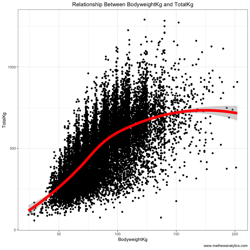
The following plot shows that the relationship between body weight and total weight lifted is fairly linear, although it flattens out around the 125 kg body weight mark.
## relationship between BodyweightKg and total weight lifted (all)

ggplot(mydat[sample(.N,20000)], aes(BodyweightKg, TotalKg)) +
       geom_point() +
       geom_smooth(method="loess", lwd=3, col="red") +
       theme_bw() +
      ggtitle("Relationship Between BodyweightKg and TotalKg") +
      labs(x = "BodyweightKg", y = "TotalKg",
      caption = "www.mathewanalytics.com") +
      theme(plot.title = element_text(hjust = 0.5))
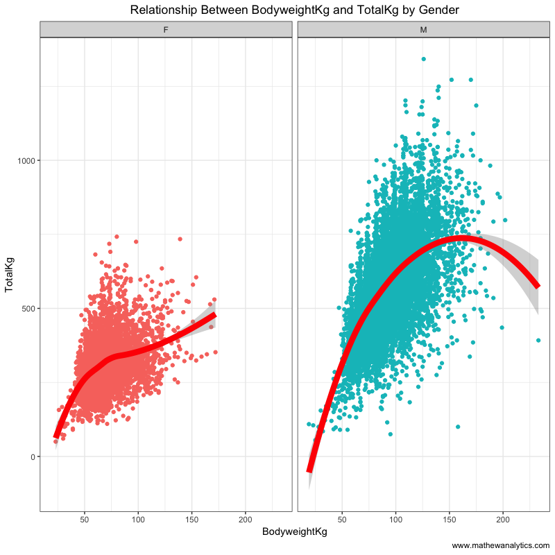
When accounting for gender in the relationship body weight and total weight lifted, we see that both share a similar trajectory.
## relationship between BodyweightKg and total weight lifted (by gender)

ggplot(mydat[sample(.N,20000)], aes(BodyweightKg, TotalKg,
       col=Sex)) +
       geom_point() +
       geom_smooth(method="loess", lwd=3, col="red") +
      theme_bw() +
      ggtitle("Relationship Between BodyweightKg and TotalKg by
      Gender") +
     labs(x = "BodyweightKg", y = "TotalKg",
     caption = "www.mathewanalytics.com") +
     theme(plot.title = element_text(hjust = 0.5)) +
     facet_wrap(~Sex)  + theme(legend.position="none")
The following scatterplot shows that peak years for powerlifters in terms of strength ranges from around age 25 to 40.
## relationship between Age and total weight lifted (all)

ggplot(mydat[sample(.N,20000)], aes(BodyweightKg, Age)) +
       geom_point() +
       geom_smooth(method="loess", lwd=3, col="red") +
       theme_bw() +
       ggtitle("Relationship Between Age and TotalKg") +
        labs(x = "Age", y = "TotalKg",
      caption = "www.mathewanalytics.com") +
      theme(plot.title = element_text(hjust = 0.5))

And here is a plot showing the distribution of total weight lifted by gender.
## relationship between Gender and total weight lifted (all)

ggplot(mydat[sample(.N,20000)], aes(Sex, TotalKg)) +
      geom_boxplot() +
      theme_bw() +
     ggtitle("Relationship Between Gender and TotalKg") +
      labs(x = "Gender", y = "TotalKg",
      caption = "www.mathewanalytics.com") +
      theme(plot.title = element_text(hjust = 0.5))

E. Regression Analysis
We are now ready to build a regression model that tries to quantify the relationship between bodyweight, age, and sex on total weight lifted. I also added a couple interaction terms to account for the interplay between bodyweight and age, and bodyweight and gender.
model_dat = mydat[, .(lifter_id, Sex, Equipment, Age, BodyweightKg,
        TotalKg, num_meets, lifter_experienced, meet_id, num_lifters,
        big_meet, prop_women, prop_women_high, AgeBucket,
        prop_old, prop_old_high, large_federation)]

dd = datadist(model_dat)
options(datadist="dd")

mod1 = ols(TotalKg ~ rcs(BodyweightKg,5) + rcs(Age,5) + Sex +
         rcs(BodyweightKg,5):Sex +
         rcs(BodyweightKg,5):rcs(Age,5),
         x=TRUE, y=TRUE, data=model_dat[!is.na(TotalKg) |
         !is.na(BodyweightKg) |
         !is.na(Age) |
         !is.na(Sex),])

mod1_pen <- update(mod1, penalty=list(simple=0,nonlinear=10),
         x=TRUE, y=TRUE)
The following plots present the predicted values of the target variable given each of the explanatory variable. Furthermore, the second plot shows the predicted values for the target variable given the interaction between bodyweight and gender. The visualization for the interaction term shows that the estimated impact of bodyweight on total weight lifted is very different given the gender of the lifter.
It seems the relationship between the target variable and Age is not linear. We can see that the highest expected value for TotalKg occurs when age is around 25 to 30. On the other hand, the relationship between the target variable and bodyweight is somewhat linear.
ggplot(Predict(mod1_pen))

plot_model(mod1_pen, type = "pred", terms = c("BodyweightKg", "Sex"))


That concludes part one of this powerlytics series where I looked to examine data on powerlifting meets in order to identify interesting patterns and trends. Part two will look at how missing a first or second attempts impacts meet outcomes.
